Lab 2026 · Real-World Production Case

Step 1 · Scenario & Setup

Engineering Role: Taking Over a Real Production Project

You join an engineering task force to audit, restructure, and optimize the logistics routing engine of a rapidly scaling company.

Your Instructor Lead Dev

I am Alban, Lead Developer at Olo Suite.

In the software industry, projects rarely arrive as clean, perfectly framed exam questions. You are usually handed a flawed legacy codebase, an incomplete customer brief, and strict business constraints that you must formalize yourselves.

Rule of the game: No turnkey solution will be given to you.
Expected mindset: Scientific rigor, critical thinking, and pragmatic software design.

Work Organization Groups of 3-4

The project is conducted in teams of 3 to 4 students:

Role 1 · Modeler / Mathematician: Rigorous problem formulation, identifying implicit constraints, and computing theoretical bounds.
Role 2 · Developer / Algorithm Engineer: Design and implementation of solving algorithms (Greedy, Local Search, LNS, OR-Tools).
Role 3 · Auditor / Data & Benchmark: Analysis of legacy solution violations, solution validation, and route visualization.

3 to 4

Students per team

4 Phases

From audit to deployment

1 Legacy

Buggy baseline solution provided

100% Real

Production-grade constraints

Overall Mission: Diagnose why the company's current solution fails miserably, lay down sound mathematical foundations, calculate incompressible lower bounds, and deliver a robust optimization engine.

Step 2 · Initial Request

The "Raw & Unfiltered" Client Brief

Here is the business requirements statement as originally drafted by operations management. It is up to you to uncover the unspoken assumptions and implicit constraints!

Excerpt from client requirements statement:
"We have 1 large central warehouse (DP) and 3 small relay hubs in the city (DS). Every morning, our heavy trucks supply the relay hubs from the warehouse. Then, small delivery vans leave the relay hubs to deliver to our customers in the city (PL). Each customer wants to be delivered within their specific time window, and some have return packages for us to collect. We want this to cost as little as possible in trucks and fuel. Here is a sketch of what we want. Figure out an algorithm for us!"

SKETCH PROVIDED BY THE CLIENT ("FLOWER" TOPOLOGY)

Distribution Network Topology

⊞ Square with Cross : Main Warehouse (DP) ⊡ Square with compact cross : Secondary Hubs (DS) ● Circles : Customer Delivery Points (PL)

Critical Brief Analysis · Did you truly understand everything?

At first glance, the problem seems deceptively simple. But as an engineer, ask yourself key questions before touching any keyboard:

Are the data and text sufficient? What implicit assumptions are left unsaid by the client?
What are the physical realities and field constraints? What happens when package flows circulate between warehouses, hubs, and customers?
What dependencies exist between network actors? Can a vehicle truly operate independently of others?
Which economic optimization criteria must you reconcile? How is overall cost measured?

Your 1st Mission · Specification & Modeling

Before writing a single line of algorithm, you must draft an impeccable mathematical and technical specification:

Formalize the problem with your own words, concepts, and equations.
Identify the exhaustive set of input parameters and decision variables.
Rigorously express the objective function and all operational constraints.
Compute and justify theoretical lower and upper bounds for the problem.

Step 3 · The Scaling Wall (Fast-Growth Crisis)

The Dilemma: "Our code worked great for 2 customers... Why is it breaking down at scale?"

The company is experiencing rapid business growth. But while their homegrown script worked perfectly during the small pilot phase, scaling up order volumes has completely jammed production. Operational costs are exploding, deliveries are arriving hours late, and management has no idea why.

🌱 Pilot Phase · Small Scale Worked Smoothly

In the early days with 1 to 2 customers (Toy Instance), the naive heuristic worked like a charm:

Trucks and vans were mostly empty (capacities were never stressed).
Delivery time windows were loose and rarely conflicted.
Vehicles arrived at hubs well ahead of van departures by pure luck.
The false illusion: Management believed their algorithm was production-ready.

💥 Production Scaling · Medium Scale Total Breakdown

As customer orders grew to 35+ (Medium Instance), the naive script hit a hard wall:

Exploding fleet: Dispatched 14 vehicles (1 truck + 13 vans!) costing €2,413.89.
Cross-dock desynchronization: Vans leave empty before trucks arrive at hubs.
Unmanageable delays: Customers waiting up to 7 hours past their promised windows.
Management's blindness: Operations cannot explain why "more orders" breaks the logic.

€2,413.89

Exploding Cost (€69 / order)

14 Vehicles

Over-provisioned Fleet (13 Vans)

27 Anomalies

Violations Detected at Scale

+454 min

Unexplained Customer Delay

Automated Audit Report (Legacy Solution on 35 PL) 27 Violations

Heavy Truck Capacity Collapse: 624 packages crammed into a 350-capacity truck at the main warehouse.
Temporal Desynchronization: Vans are dispatched at 07:30 AM from DS 2 and DS 3, but the replenishment heavy truck does not arrive until 09:23 AM and 11:19 AM!
Severe Time Window Breaches: Customer PL_29 (window closes at 10:00 AM) is delivered at 17:34 (+454 min late).
Driver Labor Limit Violations: Several van drivers spend over 10h39 on the road (legal max is 8h).

Your Diagnostic Tool · Evaluating the Failure

Run the official validator script scripts/evaluate_solution.py to inspect every single violation caused by the legacy algorithm:

Bash / Terminal

# Run the audit diagnostic on the legacy solution
python scripts/evaluate_solution.py \
  --instance data/medium_35pl/instance_medium_35pl.json \
  --solution data/medium_35pl/solution_legacy_medium_35pl.json

💡 Your Mission: Explain to management why their naive algorithm failed to scale, formulate the real mathematical constraints, and build a robust solver that scales with 0 violations and a fraction of the cost!

Inspect Legacy Code & Data: You can directly examine the legacy output file data/medium_35pl/solution_legacy_medium_35pl.json and the legacy generation script scripts/legacy_solution.py to understand the naive assumptions that caused the bottleneck.

Step 4 · Resources & Code

Datasets & Provided Toolbox

All necessary resources to get started immediately without wasting time on boilerplate infrastructure.

2D Node Map · Instance Visual Rendering (35 PL)

scripts/plot_instance.py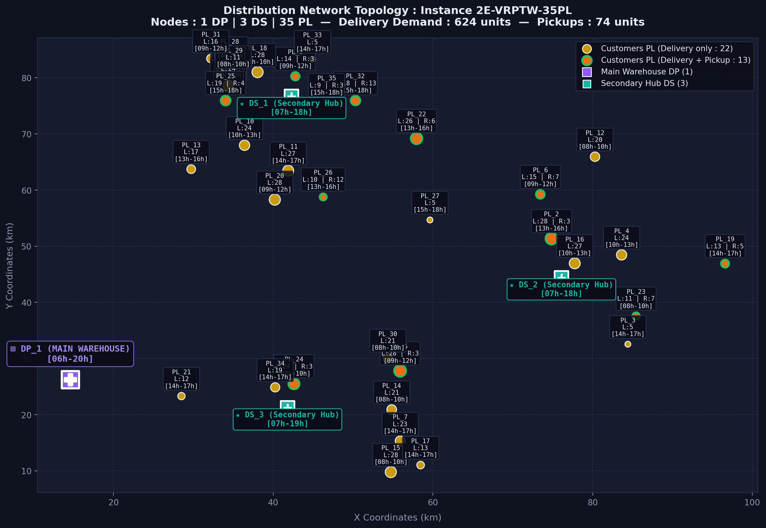

Command: python scripts/plot_instance.py --instance data/medium_35pl/instance_medium_35pl.json --show ⊞ Purple = DP | ★ Cyan = DS | ● Yellow = Delivery | 🟢 Green Border = With Pickup

Vehicle Fleet Parameters

Parameter	Tier 1 (Heavy Truck)	Tier 2 (Delivery Van)
Role	DP $\rightarrow$ DS	DS $\rightarrow$ PL
Max Capacity ($Q$)	350 units	65 units
Fixed Cost ($F$)	28 000 cts (€280.00 / day)	8 500 cts (€85.00 / day)
Variable Cost ($c$)	175 cts (€1.75 / km)	80 cts (€0.80 / km)
Max Work Duration ($T_{\max}$)	600 min (10h)	480 min (8h)

Available Files & Resources

📄 Benchmark Specification (PDF): data/docs/benchmark_instances_specification.pdf
Minimal Toy Instance (2 PL): data/toy_2pl/instance_toy_2pl.json (valid test solution)
Small Easy Instance (8 PL): data/small_easy_8pl/instance_small_easy_8pl.json (valid baseline solution)
Medium Instance (35 PL): data/medium_35pl/instance_medium_35pl.json
JSON Solution Template: data/docs/solution_template.json
Legacy Solution: data/medium_35pl/solution_legacy_medium_35pl.json
Validator Server & API: scripts/validator_server.py (Web UI + REST API)
Utility Scripts: scripts/evaluate_solution.py, scripts/plot_instance.py, scripts/load_data.py

Standardized JSON Format for Your Solution

Official Submission Schema

Any solution produced by your solver must strictly follow this structure to be accepted by the validator and API:

JSON · data/solution_template.json

{
  "team_name": "team1",
  "api_key": "sk-team1-8f3a9e2c4b",
  "instance_id": "instance_toy_2pl",
  "claimed_cost_cents": 45420,
  "routes": [
    {
      "vehicle_id": "Heavy_Truck_1",
      "stops": [
        { "node": "DP_1", "arrival": 360, "departure": 360 },
        { "node": "DS_1", "arrival": 385, "departure": 445 },
        { "node": "DP_1", "arrival": 470, "departure": 470 }
      ]
    },
    {
      "vehicle_id": "Delivery_Van_1",
      "stops": [
        { "node": "DS_1", "arrival": 460, "departure": 460 },
        { "node": "PL_1", "arrival": 472, "departure": 495 },
        { "node": "PL_2", "arrival": 510, "departure": 525 },
        { "node": "DS_1", "arrival": 537, "departure": 537 }
      ]
    }
  ]
}

🧪 Local Solution Validator 100% Client-Side · No Server Required

src/validator.js

Test and validate your solutions in real time directly on your computer. All evaluations run in-memory within your browser using pure JavaScript (or offline via the Python CLI tool). Zero server setup, zero latency.

Select Benchmark Instance:

💡 Runs client-side in memory · No network traffic

💻 Terminal & Local Python Evaluation

scripts/evaluate_solution.py

Prefer running in your terminal? The Python evaluation script runs 100% locally on your machine with standard Python 3 (no third-party dependencies):

Bash / PowerShell

# Evaluate any solution offline on your PC:
python scripts/evaluate_solution.py \
  --instance data/toy_2pl/instance_toy_2pl.json \
  --solution data/toy_2pl/solution_toy_valid.json

Minimal Starter Skeleton (Python 3)

Python 3 · scripts/load_data.py

import json

# 1. Load instance data
with open('data/medium_35pl/instance_medium_35pl.json', 'r', encoding='utf-8') as f:
    instance = json.load(f)

nodes = instance['nodes']
durations = instance['duration_matrix_min']
fleet = instance['fleet']

print(f"Loaded: {len(nodes)} available nodes (coordinates x, y available on each node).")
print(f"Total delivery demand: {instance['metadata']['total_delivery_demand']} packages")

Step 5 · Deliverables & Grading

What You Must Deliver (Deliverables & Bounds)

The project is evaluated on analytical rigor, theoretical bounds computation, code quality, and the economic performance of your final solution.

1 · The Bounds Challenge (Mandatory) Theory

Before running any solver, you must mathematically prove the incompressible boundaries of the problem:

Lower Bound on Fleet: What is the absolute theoretical minimum number of Tier 1 trucks and Tier 2 vans below which no feasible physical solution exists?
Lower Bound on Fixed Costs: What is the guaranteed baseline activation cost?
Lower Bound on Distances: How can you geometrically lower-bound the minimum distance to travel?
Upper Bound: What is the upper bound cost of an initial feasible solution?

2 · Project Roadmap & Deliverables 3 Sprints

Sprint 1 (Sessions 1 to 3) · Scoping & Modeling:
- Audit diagnostic report on the legacy solution.
- Complete mathematical specification & theoretical bounds.
- First working greedy prototype (0 validator errors).
Sprint 2 (Sessions 4 to 6) · Optimization & Metaheuristics:
- Advanced optimization engine (Local Search / LNS / OR-Tools).
- Steep cost reduction and precise relay hub synchronization.
Sprint 3 (Sessions 7 to 9) · Resilience, Benchmark & Defense:
- Handling unexpected production incidents and scaling tests.
- Final submission: Source code, route visualizations, and live presentation.

Grading Rubric (Out of 20 points)

Criterion	Points	Evaluation Expectations
1. Legacy Audit & Diagnosis	4 pts	Clear identification of the 27 violations in the legacy solution and root-cause analysis.
2. Mathematical Formalization & Bounds	5 pts	Rigor of equations, exhaustiveness of operational constraints, and soundness of lower bounds.
3. Algorithm & Solution Compliance	6 pts	Working code with strict 100% constraint satisfaction on the validator (evaluate_solution.py).
4. Economic Performance & Optimization	3 pts	Quality of cost reduction compared to legacy solution and proximity to theoretical bounds.
5. Code Quality & Visualizations	2 pts	Clean code structure, documentation, and quality of generated route plots.